Boundary Value Analysis-7

8.0 Examples: Test Cases

For each example I will show test cases for the standard Boundary Value Analysis and the Worst-case testing techniques. These will show how the test cases are performed and how comprehensive the results are. There will not be test cases for Robustness testing or robust Worst-case testing as the cases covered should explain how the process works. Too many test cases would prove to be monotonous when trying to explain a concept, however when presenting a real project when the figures are more “necessary” all test cases should be detailed and explained to their full extent. 


8.1 Next Date problem
Standard Boundary Value Analysis test cases:

                       month               day              year

                      min = 1          min = 1      min = 1812 

                     min+ = 2       min+ = 2     min+ = 1813 
                      nom = 6        nom = 15    nom = 1912 
                     max- = 11     max- = 30   max- = 2011
                      max = 12      max = 31    max = 2012

Worst-Case Analysis test cases: 

As we can see there are only 60 of 125 test cases in this example, this shows the vast amount of test cases produced.


8.2 Tri-angle problem
Standard Boundary Value Analysis test cases: 

min = 1                     

min+ = 2 

nom = 100 

max- = 199 

max = 200 

Worst-Case Analysis test cases: 

Again this is only up to 60 of 125 test cases.

Boundary Value Analysis-6

7.0 Worst-Case Testing

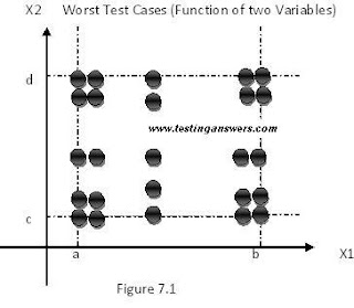
Boundary Value analysis uses the critical fault assumption and therefore only tests for a single variable at a time assuming its extreme values. By disregarding this assumption we are able to test the outcome if more than one variable were to assume its extreme value. In an electronic circuit this is called Worst Case Analysis. In Worst-Case testing we use this idea to create test cases.

To generate test cases we take the original 5-tuple set (min, min+, nom, max-, max) and perform the Cartesian product of these values. The end product is a much larger set of results than we have seen before.  

We can see from the results in figures 7.1 that worst case testing is a more comprehensive testing technique. This can be shown by the fact that standard Boundary Value Analysis test cases are a proper subset of Worst-Case test cases. 

These test cases although more comprehensive in their coverage, constitute much more endeavour. To compare we can see that Boundary Value Analysis results in 4n + 1 test case where Worst-Case testing results in 5ⁿ  test cases. As each variable has to assume each of its variables for each permutation (the Cartesian product) we have 5 to the n test cases.

For this reason Worst-Case testing is generally used for situations that require a higher degree of testing (where failure of the program would be very costly)with less regard for the time and effort required as for many situations this can be too expensive to justify.   

  

7.1  Robust Worst-Case Testing

If the function under test were to be of the greatest importance we could use a method named Robust Worst-Case testing which as the name suggests draws it attributes from Robust and Worst-Case testing.  

Test cases are constructed by taking the Cartesian product of the 7-tuple set defined in the Robustness testing chapter. Obviously this results in the largest set of test results we have seen so far and requires the most effort to produce.We can see that the function f (to calculate the number of test cases required) can be adapted to calculate  the amount of Robust Worst-Case test cases. As there are now 7 values each variable can assume we find the function f to be: 

                                  f = 7ⁿ

This function has also been reached in the paper A Testing and analysis tool for Certain 3-Variable functions [2].  

The results for the continuing example can be seen in figures 7.2

Boundary Value Analysis-5

6.0 Robustness Testing

Robustness testing can be seen as and extension of Boundary Value Analysis. The idea behind Robustness testing is to test for clean and dirty test cases. By clean I mean input variables that lie in the legitimate input range. By dirty I mean using input variables that fall just outside this input domain.  

In addition to the aforementioned 5 testing values (min, min+, nom, max-, max) we use two more values for each variable (min-, max+), which are designed to fall just outside of the input range. 

If we adapt our function f to apply to Robustness testing we find the following equation: 
                                            f = 6n + 1 

I have equated this solution by the same  reasoning that lead to the standard BVA equation. Each variable now has to assume 6 different values each whilst the other values are assuming their nominal value (hence the 6n), and there is again one instance whereby all variables assume their nominal value (hence the addition of the constant 1). These result can be seen in figures 6.1.
  

Robustness testing ensues a sway in interest, where the previous interest lied in the input to the program, the main focus of attention associated with Robustness testing comes in the expected outputs when and input variable has exceeded the given input domain. For example the NextDate problem when we an entry like the 31st June we would expect an error message to the effect of “that date does not exist; please try again”. 

Robustness testing has the desirable property that it forces attention on exception handling. Although Robustness testing can be somewhat awkward in strongly typed languages it can show up altercations. In Pascal if a value is defined to reside in a certain range then and values that falls outside that range result in the run time errors that would terminate any normal execution. For this reason exception handling mandates Robustness testing.  

Boundary Value Analysis-4

5.2 Critical Fault Assumption

The Critical Fault Assumption also known as the single fault assumption in reliability theory. The assumption relies on the statistic that failures are only rarely the product of two or more simultaneous faults. Upon using this assumption we can reduce the required calculations dramatically. 

The amount of test cases for our example as you can recall was 9. Upon inspection we find that the function f that computes the number of test cases for a given number of variables n can be shown as: 

                                          f = 4n + 1 

As there are four extreme values this accounts for the 4n. The addition of the constant one constitutes for the instance where all variables assume their nominal value. 

5.3 Generalising BVA

There are two approaches to generalising Boundary Value Analysis. We can do this by the number of variables or by the ranges these variables use. To generalise by the number of variables is relatively simple. This is the approach taken as shown by the general Boundary Value Analysis technique using the critical fault assumption.  

Generalizing by ranges depends on the type of the variables. For example in the NextDate example proposed by P.C. Jorgensen [1], we have variable for the year, month and day. Languages similar to the likes of FORTRAN would normally encode the month’s variable so that January corresponded to 1 and February corresponded to 2 etc. Also it would be possible in some languages to declare an enumerated type {Jan, Feb, Mar,……, Dec}. Either way this type of declaration is relatively simple because the ranges have set values. 

When we do not have explicit bounds on these variable ranges then we have to create our own. These are know as artificial bounds and can be illustrated via the use of the Tri-angle problem. The point raised by P.C. Jorgensen was that we can easily impose a lower bound on the length of an edge for the tri-angle as an edge with a negative length would be “silly”. The problem occurs when trying to decide upon an upper bound for the length of each length. We could use a certain set integer, we could allow the program to use the highest possible integer (normally denoted as something to the effect of MaxInt). The 
arbitrary nature of this problem can lead to messy results or non concise test cases.     

5.4 Limitations of BVA

Boundary Value Analysis works well when the Program Under Test (PUT) is a “function of several independent variables that represent bounded physical quantities” [1]. When these conditions are met BVA works well but when they are not we can find deficiencies in the results. 

For example the NextDate problem, where  Boundary Value Analysis would place an even testing regime equally over the range, tester’s intuition  and common sense shows that we require more emphasis towards the end of February or on leap years.   

The reason for this poor performance is that BVA cannot compensate or take into consideration the nature of a function or the dependencies between its variables. This lack of intuition or understanding for the variable nature means that BVA can be seen as quite rudimentary.  

Boundary Value Analysis-3

5.0 Applying Boundary Value Analysis

In the general application of Boundary Value Analysis can be done in a uniform manner. The basic form of implementation is to maintain all but one of the variables at their nominal (normal or average) values and allowing the remaining variable to take on its extreme values. The values used to test the extremities are: 

• Min ------------------------------------ - Minimal 

• Min+ ------------------------------------ - Just above Minimal 

• Nom ------------------------------------ - Average 

• Max- ------------------------------------ - Just below Maximum 

• Max ------------------------------------ - Maximum 

In continuing our example this results in the following test cases shown in figures 5.1 and 

5.2:

You maybe wondering why it is we are only concerned with one of the values taking on their extreme values at any one particular time. The reason for this is that generally Boundary Value Analysis uses the Critical Fault Assumption. There are advantages and shortcomings of this method. The advantages will be discussed in chapter 5.2, and alternative methods will be shown in chapter 7.


5.1 Some Important examples
To be able to demonstrate or explain the  need for certain methods and their relative merits I will introduce two testing examples proposed by P.C. Jorgensen [1]. These examples will provide more extensive ranges to show where certain testing techniques are required and provide a better overview of the methods usability. 

• The NextDate problem 
The NextDate problem is a function of three variables: day, month and year. Upon the input of a certain date it returns the date of the day after that of the input. 
The input variables have the obvious conditions: 
1 ≤ Day ≤ 31. 
1 ≤ month ≤ 12. 
1812 ≤ Year ≤ 2012.  
(Here the year has been restricted so that test cases are not too large). 

There are more complicated issues to consider due to the dependencies between variables. For example there is never a 31st of April no matter what year we are in. The nature of these dependencies is the reason this example is so useful to us. All errors in the NextDate problem are denoted by “Invalid Input Date.” 

• The Triangle problem 
In fact the first introduction of the Triangle problem is in 1973, Gruenburger. There have been many more references to this problem since making this one of the most popular example to be used in conjunction with testing literature.
  
The triangle problem accepts three integers (a, b and c)as its input, each of which are taken to be sides of a triangle. The values of these inputs are used to determine the type of the triangle (Equilateral, Isosceles, Scalene or not a triangle). 

For the inputs to be declared as being a triangle they must satisfy the six conditions: 
C1. 1 ≤ a ≤ 200. 
C2. 1 ≤ b ≤ 200. 
C3. 1 ≤ c ≤ 200. 

C4. a < b + c. 
C5. b < a + c. 
C6. c < a + b. 
Otherwise this is declared not to be a triangle. 

The type of the triangle, provided the conditions are met, is determined as follows: 
1. If all three sides are equal, the output is Equilateral. 
2. If exactly one pair of sides is equal, the output is Isosceles.  
3. If no pair of sides is equal, the output is Scalene.

Boundary Value Analysis-2

4.0 The Focus of BVA

Boundary Value Analysis focuses on the input variables of the function. For the purposes of this report I will define two variables ( I will only define two so that further examples can be kept concise) X1 and X2. Where X1 lies between A and B and X2 lies between C and D.  

A ≤ X1 ≤ B 

C ≤ X2 ≤ D 

The values of A, B, C and D are the extremities of the input domain. These are best demonstrated by figure 4.1. 

The Yellow shaded area of the graph shows the acceptable/legitimate input domain of the given function. As the name suggests Boundary Value Analysis focuses on the boundary of the input space to recognize test cases. The idea and motivation behind BVA is that errors tend to occur near the extremities of the input variables. The defects found on the boundaries of these input variables can obviously be the result of countless possibilities.But there are many common faults that result in errors more collated towards the boundaries of input variables. For example if the programmer forgot to count from zero or they just miscalculated. Errors in the code concerning loop counters being off by one or the use of a < operator instead of  ≤. These are all very common mistakes and accompanied with other common errors we find an increasing need to perform Boundary Value Analysis. 

Boundary Value Analysis-1

1.0 Introduction

The practice of testing software has become  one of the most important aspects of the process of software creation. When we are testing software the first and potentially most crucial step is to design test cases. There are many methods associated with test case design. This report will document the approach known as Boundary Value analysis (BVA). 

As the incredibly influential Dijkstra stated “Testing can show the presence of bugs, but not the absence”. Although this is true we find that testing can be very good at the first, if implemented correctly. For this reason we need to know of the techniques available so we can find the correct method for the system under test (SUT). 

We will look at the various topics associated with Boundary Value Analysis and use some simple examples to show their meaning and purpose. There will be some examples to show the usefulness of each method. There will be an ongoing “small scale” example to help picture each method. This will be accompanied by two examples introduced by P.C. Jorgensen [1]. These will be used to show some more “true to life” requirements for testing techniques. There will  be a chapter detailing test cases for these two more indepth examples. 

2.0 The Testing Problem

Developing effective and efficient testing  techniques has been a major problem when creating test cases; this has been the point of discussion for many years. There are several well known techniques associated with creating test cases for a system.  

There are many issues that can undermine the integrity of the result from and given test suite (set of tests) implementation. These issues or questions can be as basic as where do we start? They can become more complicated when we try to ascertain where testing should end and if we have covered all the required permutations.  

3.0 The Typing Of Languages

The typing of languages can have a large bearing on the effect of the Boundary Value Analysis approach. Strongly typed languages such as PASCAL and ADA require that all constants or variables defined must have an associated data type, which dictates the data ranges of these values upon definition. 

A large reason for languages like these to be created was to prevent the nature of errors that Boundary Value Analysis is used to  discover. Although BVA is not completely ineffective when used in conjunction with languages of this nature, BVA can be seen as unsuitable for systems created using them. 
   
Boundary Value Analysis is therefore more suitable to more “free-form” languages such as COBOL and FORTRAN which are not so strongly typed. These are also known as weak typing languages and can be seen as languages which allow one type (i.e. a String) to be seen as another (i.e. an Int). This can be useful but it can also cause bugs. These bugs or errors are normally found in the ranges that BVA operates in and therefore can find.